$\def\bm#1{{\boldsymbol{#1}}}
\def\coloneqq{{:=}}
\def\mathbbm#1{{\mbox{#1}\hspace{-0.20em}\mbox{l}}}$

Yang-Baxter 方程式

$6$頂点模型の$R$行列は

\begin{equation}
R=\left(
\begin{array}{cccc}
a&0&0&0\\
0&b&c&0\\
0&c&b&0\\
0&0&0&a
\end{array}
\right)
\end{equation}

とあらわされる。以下では$2$つのパラメーター$\eta\in\mathbb{C}$（anisotropy parameter）、$u\in\mathbb{C}$（spectral parameter）を用いる。これによって

\begin{equation}
(a,b,c)=(\sin{(u+\eta)},\sin{u},\sin{\eta})\tag{1}
\end{equation}

とあらわされる場合、及びその極限をとった

\begin{equation}
(a,b,c)=(u+\eta,u,\eta)\tag{2}
\end{equation}

とあらわされる場合を考察する。(1)の場合の行列$R$のことをtrigonometric matrix といい、(2)の場合の行列$R$のことをrational matrix という。以後、$u$依存性を強調して$R(u)$と書くことがある。

さて、(1)、(2)の場合、$R$行列において
\begin{equation}
R_{12}(u_1-u_2)R_{13}(u_1-u_3)R_{23}(u_2-u_3)=R_{23}(u_2-u_3)R_{13}(u_1-u_3)R_{12}(u_1-u_2)\tag{3}
\end{equation}
が成り立つ。これをYang-Baxter 方程式という。但し、$R_{12}(u),R_{13}(u),R_{23}(u)\in\mathrm{End}(V_1\otimes V_2\otimes V_3)$、及び$V_i\simeq\mathbb{C}^2$である。

次に成分表示について考えよう。$R(u_i-u_j)^{ab,lm}=r_{ij}^{ab,lm}$と書くと、(3)は

\begin{equation}
r_{12}^{a_1c_1,a_2c_2}r_{13}^{c_1b_1,a_3c_3}r_{23}^{c_2b_2,c_3b_3}=r_{23}^{a_2c_2,a_3c_3}r_{13}^{a_1c_1,c_3b_3}r_{12}^{c_1b_1,c_2b_2}
\end{equation}

となる。これを絵で描くと次のようになる。

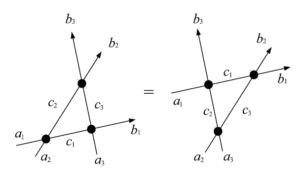
図19 $6$頂点模型の略記図

(2)の場合の証明について考えよう。

\begin{align}
R=&R(u)=\left(
\begin{array}{cccc}
u+\eta&0&0&0\\
0&u&\eta&0\\
0&\eta&u&0\\
0&0&0&u+\eta
\end{array}
\right)=u\left(
\begin{array}{cccc}
1&0&0&0\\
0&1&0&0\\
0&0&1&0\\
0&0&0&1
\end{array}
\right)+\eta\left(
\begin{array}{cccc}
1&0&0&0\\
0&0&1&0\\
0&1&0&0\\
0&0&0&1
\end{array}
\right)\nonumber\\
=&u(\bm{1}\times\bm{1})+\eta P
\end{align}
但し、$P$は$P(x\otimes y)=y\otimes x$を満たすことを思い出しておくこと。従って、(2)左辺を$x\otimes y\otimes z\in V_1\otimes V_2\otimes V_3$を用いて変形していくと

\begin{align}
&R_{12}(u_1-u_2)R_{13}(u_1-u_3)R_{23}(u_2-u_3)(x\otimes y\otimes z)\nonumber\\
=&R_{12}(u_1-u_2)R_{13}(u_1-u_3)\{(u_2-u_3)(x\otimes y\otimes z)+\eta(x\otimes z\otimes y)\}\nonumber\\
=&(u_1-u_2)(u_1-u_3)(u_2-u_3)(x\otimes y\otimes z)+(u_1-u_3)(u_2-u_3)\eta(y\otimes x\otimes z)\nonumber\\
&+(u_1-u_2)(u_2-u_3)\eta(z\otimes y\otimes x)+(u_1-u_2)(u_1-u_3)\eta(x\otimes z\otimes y)\nonumber\\
&+(u_2-u_3)\eta^2(y\otimes z\otimes x)+(u_1-u_3)\eta^2(z\otimes x\otimes y)+(u_1-u_2)\eta^2(y\otimes z\otimes x)+\eta^3(z\otimes y\otimes x)\nonumber
\end{align}

問題11

上と同様に(2)の右辺を$x\otimes y\otimes z$に作用させたものに計算し、(3)の右辺と同じになることを確かめよ。

解答11

題意に沿った計算では、
\begin{align}
&R_{23}(u_2-u_3)R_{13}(u_1-u_3)R_{12}(u_1-u_2)(x\otimes y\otimes z)\nonumber\\
=&R_{23}(u_2-u_3)R_{13}(u_1-u_3)\{(u_1-u_2)(x\otimes y\otimes z)+\eta(y\otimes x\otimes z)\}\nonumber\\
=&R_{23}(u_2-u_3)\{(u_1-u_3)(u_1-u_2)(x\otimes y\otimes z)+\eta(u_1-u_2)(z\otimes y\otimes x)\nonumber\\
&+\eta(u_1-u_3)(y\otimes x\otimes z)+\eta^2(z\otimes x\otimes y)\}\nonumber\\
=&(u_2-u_3)(u_1-u_3)(u_1-u_2)(x\otimes y\otimes z)+\eta(u_1-u_3)(u_1-u_2)(x\otimes z\otimes y)\nonumber\\
&+\eta(u_2-u_3)(u_1-u_2)(z\otimes y\otimes x)+\eta^2(u_1-u_2)(z\otimes x\otimes y)+\eta(u_2-u_3)(u_1-u_3)(y\otimes x\otimes z)\nonumber
&+\eta^2(u_1-u_3)(y\otimes z\otimes x)+\eta^2(u_2-u_3)(z\otimes x\otimes y)+\eta^3(z\otimes y\otimes x)\nonumber
\end{align}
よって題意は示された。

次に転送行列の可換性について考えよう。Yang-Baxter 方程式の帰結として、以下の性質が知られている。
\begin{equation}
V=\mathbb{C}\leftarrow\oplus\mathbb{C}\rightarrow　,　\mathcal{H}=W_1\otimes\cdots\otimes W_M　,　W_i=\mathbb{C}\uparrow\oplus\mathbb{C}\downarrow
\end{equation}
として、$T(u;z)$を以下のように定義する。
\begin{equation}
T(u;z)=T(u;z_1,\cdots,z_M)\in\mathrm{End}(V\otimes\mathcal{H})　,　T(u;z)=L_M(u-z_M)\cdots L_1(u-z_1)
\end{equation}
$T(u;z)$のグラフによる表示は以下のように描ける。

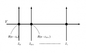
図20 $6$頂点模型の略記図

ここでYang-Baxter 方程式を用いると
\begin{equation}
T_{23}(v;z)T_{13}(u;z)R_{12}(u-v)=R_{12}(u-v)T_{13}(u;z)T_{23}(v;z)\tag{4}
\end{equation}
が成立する。但し、$T_{23},T_{13},R_{12}\in\mathrm{End}(V_1\otimes V_2\otimes\mathcal{H}),V_i\in\mathbb{C}\rightarrow\oplus\mathbb{C}\leftarrow$となる。(4)のグラフによる表示は以下のように描ける。

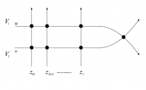
図21 $6$頂点模型の略記図

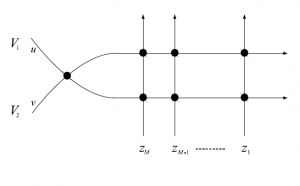
図22 $6$頂点模型の略記図

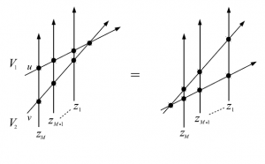
図23 $6$頂点模型の略記図

(4)の証明のためには、Yang-Baxter 方程式を利用する必要がある。Yang-Baxter 方程式を絵で描いた、図19のような変換を順番に施していけば、絵的に証明を行うことが出来る。

他にすぐ分かる性質として、転送行列の可換性がある。$\mathcal{T}(u;z)=\mathrm{Tr}_VT(u;z)$に関して、
\begin{equation}
\mathcal{T}(u;z)\mathcal{T}(v;z)=\mathcal{T}(v;z)\mathcal{T}(u;z)\tag{5}
\end{equation}
が成立する。これは転送行列が可換であることを意味している。この結果から、$6$頂点模型は対称性が極めて高い、非常に特殊な設定であるということが分かる。

(5)の証明を行なおう。(4)より、
\begin{equation}
R_{12}(u-v)T_{13}(u;z)T_{23}(v;z)R_{12}(u-v)^{-1}=T_{23}(v;z)T_{13}(u;z)
\end{equation}
となる。この式の両辺において、$V_1\otimes V_2$について部分トレースを取ると、
\begin{align}
(左辺)=&\mathrm{Tr}_{V_1\otimes V_2}(R_{12}(u-v)T_{13}(u;z)T_{23}(v;z)R_{12}(u-v)^{-1})=\mathrm{Tr}_{V_1\otimes V_2}(T_{13}(u;z)T_{23}(v;z))\nonumber\\
\overbrace{=}^{(*)}&\mathcal{T}(u;z)\mathcal{T}(v;z)
\end{align}
となる。右辺も同様にして、$\mathrm{Tr}_{V_1\otimes V_2}(T_{23}(v;z)T_{13}(u;z))\overbrace{=}^{(*)}\mathcal{T}(v;z)\mathcal{T}(u;z)$となる。

問題12

$(*)$を確かめよ。

解答12

今、$\mathcal{T}(u;z)=\mathrm{Tr}_VT(u;z)$、$T_{23},T_{13}\in\mathrm{End}(V_1\otimes V_2\otimes\mathcal{H})$だから、これらより
\[
\mathrm{Tr}_{V_1\otimes V_2}(T_{13}(u;z)T_{23}(v;z))=\mathcal{T}(u;z)\mathcal{T}(v;z)
\]
となる。